In Part 1, I discuss growth in games and the definition of an engine building game. In Part 2, I will discuss player odds and the problem of engine building games, as well as the consequences of specific quantitative properties of engine building games. In Part 3, I will discuss additional solutions to the problem of player odds.

Diverging Player Odds

In Characteristics of Games, the authors discuss the concept of tracking players’ probabilities of winning at various points in a game. If a game is designed in such a way that those probabilities of winning diverge too quickly, players will probably have limited motivation to continue playing. For instance, if 10% of the way through a game, it were consistently obvious who would win the game, this game might be considered flawed (especially if, like most multiplayer games, players were not allowed to concede the game early!) On the other hand, if a game were such that the probabilities of each player winning consistently remained too close together for the majority of the game, that would mean that players’ early game performance were meaningless, and players would likely notice this. For instance, in a four-player game wherein no matter what players did for the first 90% of the game, each player still had about 25% chance of winning going into the last 10% of the game, the first 90% of the game would seem pointless. Therefore, the divergence of the winning probabilities for each player should ideally have some moderate rate, although the “best” rate is not currently known to us, and could be further studied.

Player Odds

For the purpose of the visualizations and some of the analysis I will do in this article, it is useful to think about players’ odds of winning. Odds are simply a different way of expressing a player’s probability of winning. Instead of saying that a player has a 90% chance of winning, we can say he has 9:1 odds. If the player has a 1% chance of winning, his odds are 1:99 or 1/99. Because odds tend to grow exponentially as the game progresses (even in linear games), it is useful to look at players’ log odds. This mathematical transformation of a player’s odds puts the odds on a scale that’s easier for people to see and understand. For the rest of the article, whenever I use the word “odds,” I will be referring to “log odds.” Here is a guide for how we can interpret a player’s log odds:

Log Odds	Win Probability	Interpretation
> 4	> 98%	Effective Victory
3	95%	Dominating
2	88%	Winning
1	73%	Advantaged
0	50%	Tied
-1	27%	Disadvantaged
-2	12%	Losing
-3	5%	Hopeless
< -4	< 2%	Effective Elimination

Therefore we would hope that a player’s log-odds would tend to stay between -3 and 3 throughout most of the game. Once a player’s odds diverge past 4 or -4 or so, they will likely lose interest in the competitive aspect of the game.

Odds Diagrams

Let’s visualize the relationship between players’ odds and T, the amount of time which has elapsed in a game. We can’t directly measure this for real games, because we can’t fully calculate a player’s chances of winning, but we can do an analysis of this sort of some contrived archetypal games. Here I plot what I call odds diagrams for basic types of games in which two players score points randomly. Of course in real games players also have to make decisions, but for the purpose of this article I am including the variability in outcomes of players’ decisions in the overall variability of their performance. Here I model the totality of that variability using probability distributions. Thus these models approximate situations in which two players of equal skill are playing a highly complex game, and the utility of their decisions varies randomly due to the difficulty of the game.

Linear Games

In this first archetypal game, each round, each player scores a random number of points using the same random number generator each time. (In real life, players would probably use dice, but I for the ease of computation I use Gaussians to make these plots). Because players are endowed with constant-valued assets proportional to the time remaining in the game, this is therefore a linear game.

Let’s plot the odds curves for the players of this random game if there are 10, 20 or 30 rounds.

In these plots, the upper curve is the average odds for the player who will win the game, and the lower curve is the average odds for the player who will lose the game.

The horizontal lines demarcate the subjective regions of player odds I named above. While player odds remain between the green lines, both players most likely feel like they are “still in the game.” Once the odds diverge past the red lines, the losing player most likely feels like his position is irredeemable

We can see that in this linear game between two equally skilled players, player odds stay within acceptable margins for most of the game. Only in the last 20% of the game do odds diverge to the point where the game is decided.

Furthermore, we can see that the curves have the same shape in each case – in linear games, it’s just as easy to catch up as it is to fall behind, so the game length doesn’t have an impact on the divergence of the player odds.

Let’s experiment by changing the amount of variability in player outcomes. Consider variants of this game where the individual outcomes have low, medium and high variability. For instance, a relatively low variability game would be one in which players roll D6s, whereas a relatively high variability game would be one in which players roll D100s. 

 

 

Again, the curves are identical. Once again this is because higher variability identically affects players abilities to fall behind and catch up, and thus has no impact on the overall shape of the odds curves.

Linear games seem to be fairly stable entities, and although I can’t say what shapes of odds-curves are most desirable in games, I would guess that the curve exhibited by these linear games is within acceptable margins, at least for similarly skilled players.

Exponential Games

However, if we look at exponential games, things get a bit hairier. This second game is a random exponential game. Player score a random number of points on each round, and then these points are invested so that they yield an exponential rate of return throughout the game. Thus, if a player scores a certain number of points in a particular round, these points are then amplified by a factor of e^cT, where T is the number of turns left in the game and c is the relative growth rate of the game.

Let’s compare the odds curves associated with this game to the odds curves associated with a linear game.

In these plots, the blue curves represent the odds curves from a linear game as before, and the red curves represent the odds curves from exponential games which exhibit varying levels of relative growth.

When c = 0, the exponential game is the same as the linear game. However, as c increases, the odds curves of the exponential game begin to diverge much more rapidly. This is because outcomes from the early rounds are disproportionately impactful on the outcome of the game. The higher the investment factor c, the more the value of early game outcomes dominates the value of late game outcomes, thus the earlier the game is decided.

Remember that these odds are on a log scale; in the exponential game with c = .1, a clear winner emerges just over halfway through the game. Thus as we increase the investment factor rate of growth of a game, odds begin to diverge much more rapidly.

Furthermore, in an exponential game, game length has a real effect on the shape of odds curves. Let’s exam the behavior of odds curves for exponential games at different game lengths.

As we can see, the longer the game, the faster player odds diverge relative to the length of the game. This is because investments have longer to mature, and thus early game successes are of more profound importance.

Thus, in some sense, exponential games are not robust to changing game length. Meanwhile, a linear game could be extended to 100 turns without losing stability.

 

Solutions to the Problem of Diverging Odds

Now that I have argued that exponential player growth in games can cause undesirably fast divergence of players’ probabilities of winning, I can use this to explain many of the attributes of modern games. Games exhibit exponential growth because it is desirable, but must introduce further mechanisms to address the undesirable possibility of logical player elimination. Here I propose that there are five categories of solutions which games use to deal with this problem, which are:

1. Restraint Mechanisms (which reign in or counteract player growth)
2. Damping Mechanisms (which coerce player standings into similarity)
3. Variance Reduction Mechanisms (which reduce variation in player’s individual outcomes)
4. Escalation (which delays the divergence of player odds)
5. Obfuscation Mechanisms (which obscure logical player elimination).

Solution 1: Restraint Mechanisms

For the remainder of Part 2 I will discuss the category of solutions which is specific to engine building games.

This first and most important category of solutions to the problem of too-quickly diverging odds in engine building games is simply to introduce mechanisms into the game which prevent players from growing too dramatically. As we established, diverging player odds in exponential games are driven by early game differences in player performances becoming amplified by exponential growth. If we restrain this growth, then we reduce the amplification of early differences in player performances.

In this section I will discuss ways in which games manipulate the parameters of assets’ exponential growth in order to prevent them from causing rapid divergence in player odds. First I propose a way of modelling the value of exponential assets. We can very roughly model the value of exponential assets as:

ke^cT – p(k,c,T), where

• k is the “scaling” factor which can increase or decrease the value of exponential assets relative to similarly available constant-type assets. By decreasing k, games can downweight the importance of the exponential assets and make constant-type and linear-type alternatives more viable.
• c is the “relative growth rate” of the exponential asset. Assets with a high “c” value will grow very quickly, and with a low “c” value will grow very slowly.
• T is the time remaining in the game. Long games will result in overwhelming exponential assets, whereas short games don’t give assets much time to grow.
• p(k,c,T) is a penalty function, which may depend on k, c and T, but which is sub-exponential. Penalty functions come in many forms, but are essentially costs that player incur which disincentive exponential assets.

By manipulating these four parameters of exponential assets, games can restrain their growth. In the following sections, I will look in depth at how games manipulate each of these four parameters.

Scaling (Reducing “k,” the scaling factor)

The first strategy to reduce the potency of exponential assets in games is to simply scale down the total value of these assets.

If  exponential assets have great value relative to players’ endowments and similarly available constant and linear-type assets, players are compelled to invest in them and any variability in players’ outcomes in this regard will be amplified, resulting in diverging player odds. If exponential assets have minor value relative to their alternatives, their impact on players’ odds are limited.

Consider a game in which players can gain either rabbits or mules. Rabbits double in number each round, but mules do not. At the end of the game, rabbits are worth some number of points and mules are worth some other number of points. Depending on the length of the game, the value of rabbits should be a fraction of the value of mules in order to keep the decision between rabbits and mules meaningful. A game which lasts 5 rounds, in which value of a rabbit is equal to the value of a mule, will result in a huge amount of divergence in player odds, assuming there is any variability in whether a player can gain a rabbit or a mule, and when (as I will discuss in the section on variance reduction). In a game which lasts 5 rounds, but in which rabbits are given a value of 1/100 that of mules, rabbits are consistently a suboptimal choice, and thus their existence in the game is likely superfluous but will not result in diverging player odds. Being stuck with a rabbit may be suboptimal, but this will have a less dramatic linear-type impact on diverging player odds, rather than an exponential-type impact.  

As a real example, consider Isle of Skye, which is overall at most a quadratic game (in that players gain linear-type assets which pay off in victory points steadily over time), except for the existence of “whiskey barrel” tiles which increase a player’s income by 1.

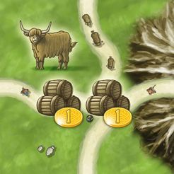
 The magnitude of this increased income is minute compared to a player’s base income of 5, as well as the endowments players receive in the form of tiles to sell each round. We can imagine a scaled-up version of this mechanism, in which each whiskey barrel tile increases a players’ income by 5 instead of 1. In that case, the value of these barrel tiles would dominate the value of all other tiles early in the game, and whether or not players were able to gain these tiles early would determine their success in the game. Thus we can see that this choice of scaling suppresses the impact of an exponential mechanism on the outcome of the game.

Slowing (Reducing “c,” the relative growth rate)

It becomes clear that scaling can’t entirely fix the Rabbit and Mule game, because having an asset which doubles in value each round is rather unstable. Even in a properly scaled game, in one round rabbits will utterly dominate the value of mules, and some rounds later the value of mules will utterly dominate the value of rabbits. It seems we need to reduce the reproduction rate of rabbits. In doing so we would be reducing the parameter “c,” the relative growth rate of the rabbits. Instead of rabbits doubling every round, we could have them grow by a factor of 1.5 (each pair of rabbits has one baby each round) or 1.414 (the rabbits double in number only once every other round).

Take for instance Terraforming Mars which is an engine building game which lasts over the course of 12-15 rounds. The 12-15 opportunities for income leave room for a huge amount of growth (the game has a high “T”), so the game compensates for this in part by keeping the relative rate of growth low. Players are endowed with about 50 units of starting resources, and it is common on the first round for a player to spend all of his initial resources to increase his income by only the equivalent of 2-5 units. Because the price of increasing one’s income is high, players increase their income relatively slowly. One can imagine if it only cost about 5 units of currency to increase one’s income by 1, it were common for players to gain 8-15 income in the first round; those who gained only 8 income would very likely lose hope in the subsequent rounds as those who gained 15 income pulled ahead. The overall growth factor would be exponentially greater, and odds would diverge extremely quickly. (In Terraforming Mars, this slowing is especially important due to players’ random options; I will discuss this further in the section on variation reduction.)

Since exponentially growing assets in games sometimes act in discrete and contextual ways, slowing isn’t always quite as easy as turning a dial to adjust a parameter. In A Feast for Odin, Uwe Rosenberg rather transparently slows the growth of Cattle and Sheep by dictating that they reproduce only once every other round, rather than once per round. Many games slow exponential growth by limiting options for player to invest and forcing players to space out investments over time by requiring that they jump through hoops in order to make them.

Games sometimes also encourage players to fight over opportunities for exponential growth. For instance, in Stone Age, there is only one space available for players to gain an extra family member, and it is desirable enough that players can’t expect to be able to take it every round. Similarly, in Agricola, even if a player very quickly builds a house which can support 5 family members, she likely won’t be able to grow her family every round if other players are still in contention to grow their own families. If players are forced to space out their acquisition of exponential assets, this will naturally slow their growth rates (a la rabbits reproducing only every other round or so).

Growth is limited not only by the price of investments (and thus the amount that resources can propagate), but also the accessibility of those resources and the delays necessitated by their acquisition. Consider Alien Frontiers, a dice-placement game in which players must place dice showing a pair in order to spend some energy and some ore at the shipyard in order to gain additional dice; meeting all of these criteria is likely to take 2-4 turns, thus slowing down the rate at which players may gain dice. Similarly, the dual resource cost delays the building of houses in Agricola, and gaining extra workers in Russian Railroads involves jumping through various and time-consuming hoops.

Stopping (Reducing “T,” the game length)

Recall that the driving exponential factor in our asset growth model is e^cT. So in addition to slowing the growth of assets by reducing c, we can reduce the potency of assets by reducing T, the length of the game. Essentially, the shorter a game is, the less time players have to grow, and thus the less their early performances will be amplified. This concept, combined with the assumption that modern board games aim to limit the divergence of player odds, explains why engine building games tend to end just a moment before players can derive the satisfaction of utilizing their engine to the extent they desire.

Revisiting the Rabbit and Mule game, we have seen that it is important to consider the length of the game when implementing the scaling and growth rate of the rabbits. When should the Rabbit and Mule game end? I posit that it should end at a time such that an early game acquisition of Rabbits is more valuable than an early game acquisition of mules. If it doesn’t, then Mules are unilaterally better than Rabbits, and why include Rabbits in the game at all? (I’ll write about this often-discussed principle of parsimony in games in a later article). However, if the game ends too long after the value of Rabbits surpasses that of Mules, the game will be highly volatile and any variability in players’ acquisition of Rabbits will be heavily amplified.

Indeed, players who wish that games were just “one round longer,” so that they could watch their engines satisfyingly take off, should be careful what they wish for. In such a game, players would be robbed of the rare delight of achieving surprising and spectacular results because this would be the norm. Furthermore, at this point in the game, exponential assets begin to utterly dominate all other types of assets, thus players likely know who has won and continuing to play may be pointless.

For example, Race for the Galaxy is highly exponential but relatively short. If the game were extended by 25%, I hypothesize that far fewer games would end in suspense, and player concession would be much more frequent. In a two-player game, imagine a player who chooses the low-growth strategy of producing and consuming one good per turn for two points; this player will end up with about 18-25 points, whereas his opponent who plays the game properly by building a productive tableau might win with a score of about 30-40. 

If the game were two rounds shorter, this growth-oriented player would likely lose, which would render most of the mechanisms of the game pointless. Thus Race for the Galaxy ends appropriately after the value of exponential assets surpasses that of linear-type assets, but before players’ average odds diverge to the point of futility. 

Similarly, Dominion is moderately exponential but relatively short; Terraforming Mars is long but exhibits slower growth than these previous examples. Games which are long and highly exponential, like Power Grid or Agricola, will need other techniques to ensure player odds don’t diverge too quickly.

Penalizing

Finally, games can reduce the overwhelming value of exponential assets in exponential games by attaching a penalty to their acquisition. I write the penalty term in my exponential asset model as p(k,c,T) because this penalty may depend on the value of the asset itself, including its scaling, its growth rate, and the amount of time left in the game. I will focus on constant-type penalties (which do not depend on T) and linear-type penalties (which have a magnitude which depends linearly on T), as exponential penalties may best be modeled as the trading of one exponential asset for another.

We might further modify the game of Rabbit and Mule so that players incur a penalty for acquiring Rabbits. For instance, we could dictate that whenever a player gains a Rabbit, he loses 5 points; this would constitute a constant-type penalty it does not depend on the time remaining in the game. Or, we could penalize players who gain rabbits in a linear way; for instance we could implement a rule which says that whenever a player takes a move to gain a new rabbit, he incurs a penalty of 1 point per round for the rest of the game. In either case, we could somewhat increase some combination of k, c, and T, (the scaling of the rabbits, the growth rate of the rabbit, and the time remaining in the game), but retain the competitive values of mules and rabbits.

For a real but similarly agricultural example, consider Agricola, in which players who grow their family must pay two food in each harvest for the rest of the round. 

Food in Agricola can technically be used as currency, but I would argue that it should largely be considered a constant-valued asset, as its primary purpose is to avoid constant-valued negative-point begging cards. Therefore feeding acts as a linear penalty against player growth. Feeding in Tzolk’in and other games with “feed your workers” mechanisms functions similarly.

Constant-type penalization is common in games with mixed assets like Race for the Galaxy. Cards are at generally worth points commensurate with their cost in discards. However, assets which have a high exponential (or linear) value will often be tempered by a reduction in constant value. 

 

 

This concludes the discussion of the first of five solutions to the problem of diverging odds in engine building games. In Part 3 I discuss the remaining four more general solutions to diverging odds, and conclude the article.